Procedural Generation For Dummies: Road Generation In Which Tractable Tensors Are Traced Terrifically
Procedural City Generation For Dummies Series
- Procedural Generation For Dummies: Building Footprints
- Procedural Generation For Dummies: Half Edge Geometry
- Procedural Generation For Dummies: Galaxy Generation
- Procedural Generation For Dummies: Lot Subdivision
- Procedural Generation For Dummies
- Procedural Generation For Dummies: Road Generation
My game, Heist, is a cooperative stealth game set in a procedurally generated city. This series of blog posts is an introduction to my approach for rapidly generating entire cities. If you’re interested in following the series as it’s released you can follow me on Twitter, Reddit or Subscribe to my RSS feed
A lot of the code for my game is open source - the code applicable to this article can be found here. Unfortunately it has some closed source dependencies which means you won’t be able to compile it (I hope to fix that soon) but at least you can read along (and criticise my code).
Road Generation
The majority of road generation systems I have looked at tend to be based on a growth system. The general algorithm (see page 15, Section 3.2 of this paper) for pretty much all of them is pretty simple.
- Keep a priority queue of candidate road segments
- Initialised with a single seed segment
- While priority queue is not empty
- Remove highest priority segment from queue
- Check local constraints on segment
- This may modify the segment, or even reject it
- Add segment to output
- Generate new segments (connected to this segment) based on global goals
Or in pseudo code:
//Create a priority queue of things to process, add a single seed
let Q : priority queue;
Q.Add( 0, seed );

//Create a list of segments (the result we're building)
let S : segment list;

while !Q.IsEmpty()
{
    //Remove the highest priority item from the priority queue
    let t, segment = Q.RemoveSmallest();

    //Check that it is valid, skip to the next segment if it is not
    let modified = CheckLocalConstraints(segment);
    if (modified == null)
        continue;

    //It's valid, so add it to S. It is now part of the final result
    S.Add(segment);

    //Now produce potential segments leading off this road according to some global goal
    for (tn, sn) in GlobalGoals(segment)
        Q.Add(t + tn + 1, sn);
}
Hopefully this is fairly clear. We simply generate a load of candidate points (in the GlobalGoals function), add them to a priority queue and then accept or reject each individual segment (in the CheckLocalConstraints method). The real variety between different algorithms comes in how you generate new constraints and how you express your global goals.
Global Goals
This is our method for producing new segments according to large scale global goals. For example one possible implementation would be to generate a single new segment at the end of the input segment which leads towards the local population centre. This would generate you one long road which leads from your random seed point directly to the population center and then stops.
The critical part of this method is that it generates segments with no concern for if they are possible. This means global goals can be very fast and simple to implement.
Local Constraints
This is our method for accepting, rejecting and modifying individual segments according to small scale local constraints. For example we could come up with a set of rules such as:
- If a candidate segment crosses another segment then join the roads together to form a T-Junction.
- If a candidate segment stops near to another segment then extend it to join the roads and form a T-Junction.
- If a candidate segment stops near an existing T-Junction then extend it to join the junction and form a cross-junction.
As you can see these rules are all about correcting small errors to improve the local consistency of the road network.
Tremendous Tensors
My implementation is based off the paper Interactive Procedural Street Modeling (Chen, Esch, Wonka, Mueller, Zhang, 2008). If you’re not up for reading the paper then there’s a short (5 minute) video here with an overview of the technique.
How this systems works is twofold. First you generate a tensor field (if you don’t know what a tensor is don’t worry about it - in this system the tensors are just 2 dimensional vectors) and then you trace lines through the field (following the tensors).
Every tensor in this system has two eigen vectors (once again, if you don’t know the exact mathematical definition don’t worry about it). The two eigen vectors are always perpendicular and we’re going to refer to them as major and minor. We do the tracing through the field twice - once along the major vectors and once along the minor vectors.

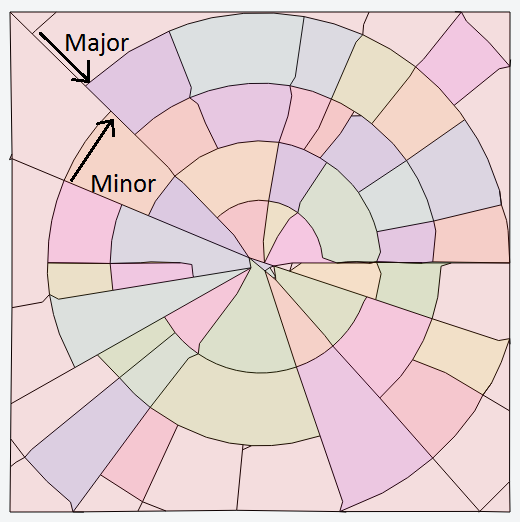

So what use are these tensor fields? Above you can see a tracing of the most basic tensor field - a grid. This is simply the same tensor repeated everywhere and since the major and minor vectors of the tensor are perpendicular we end up with a grid! The paper defines several methods for generating tensor fields for different situations:
- Grid
- Major points across grid.
- Minor points along grid.
- Radial
- Major points to centre.
- Minor points around centre
- Heightmap
- Major points along gradient.
- Minor points across gradient
- Polyline
- Major points to nearest point on path.
- Minor points along path
The really cool thing about tensors is that we have ways to easily combine them. If you have multiple tensor fields it turns out that if you simply take a weighted average of all the fields you end up with a sensible result which you can trace. If your weight is set to fall off with distance you can define different tensor fields in different locations and they will slowly blend together as the weight changes!
Here’s a far more complex road network, generated by blending together multiple different fields:
- Grid Top Left
- Grid Top Right
- Grid Bottom Left
- Grid Bottom Right
- Radial Centre
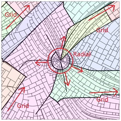
You can clearly see the five different elements and how the roads smoothly transition from following one to following the next.
Implementation Details
As mentioned at the start of the article the source code for my implementation of this system is here. The specific code for tracing through tensor fields and building a road network is here.
Before I dive into details I should say that this implementation is one of the parts of the city generation system I am most unhappy about. Tracing vectors is extremely sensitive to errors because the errors accumulate along the entire length of the streamline. Additionally the tracing can be quite slow, most of the example images in this post took 5-10 seconds to generate (which isn’t unusably slow, as we only need to do this step once per city).
Design Your Tensor Field
The first step is to build a tensor field. Right now I’m just doing this by hand but ultimately I’d like to do this automatically - for example:
- Cover the entire map with a heightmap conforming tensor field
- Place gridlines/radials at major population centres
- Place a polyline along any major terrain features such as rivers or cliffs
In my implementation I have a base interface for tensor fields which can be sampled at any point. I then have multiple concrete implementations for different tensor field types.
Once the tensor field is created I have a single step which converts the tensor field into an eigen field. An eigen field is simply just a pair of vector fields along the eigen vectors; one along the major eigens and one along the minor eigens. This conversion process samples the tensor field (which a fairly expensive process with a lot of mathematical operations) at set intervals and caches the value. This caching more than tripled the speed of the overall system!
Trace Your Vectors
Now we have two vector fields, we need to trace a line through these fields, a streamline. Conceptually tracing through a vector field is trivial:
let point = start
until (some end condition)
    let direction = sample_vector_field(point)
  point += direction
However this turns out not to work very well. Because this only samples one single point from the field it is extremely sensitive to local noise and does not work at all when the field is highly curved (e.g. around a radial field). Instead I use an RK4 integrator to handle the higher curvature (see this excellent article for more details on integration):
function rk4_sample_vector_field (point)

    let k1 = sample_vector_field(point)
    let k2 = sample_vector_field(point + k1 / 2f)
    let k3 = sample_vector_field(point + k2 / 2f)
    let k4 = sample_vector_field(point + k3f)

    return k1 / 6f + k2 / 3f + k3 / 3f + k4 / 6f
Another problem to handle is that when we’re tracing through the field we don’t care about positive or negative direction - a gridline left to right is the same as a gridline right to left. I handle this by again modifying how I sample the vector field. When a sample is taken it compares the direction of the sample to the direction of the previous vector; if they differ by more than 90 degrees the direction is reversed:
function corrected_sample_vector(point, previous_direction)

    # Sample the vector field, For real this time!
    let sample = sample_vector_field(point)

    # If previous is zero that's a degenerate case, just bail out
    # Dot product >= zero indicates angle < 90
    if (previous_direction == Vector2.Zero || Dot(previous_direction, sample) >= 0)
    return v;

    # Since we didn't return one of the cases above, reverse the direction
    return -v;
Back To Basics
How does this all fit into the algorithm I outlined at the top? This vector tracing is effectively the Global Goals function - a single streamline is a collection of candidate segments to add into the map. The global goals in this case are the underlying tensor fields.
How we handle the line segments traced through the vector field is our Local Constraints function.
Rather than keeping a buffer of all the segments of a streamline and handling them one by one, an entire streamline is traced out and stops when a segment is rejected - this is just an optimisation to save a load of bookkeeping work. You can see the method which traces streamlines here and the method which creates each segment (and checks constraints) here.
If any of these conditions is met the streamline is stopped:
- Segment is too short
- Segment reaches the edge of the map
- Segment ends very near an existing vertex
- Connect end of streamline to that vertex
- Segment intersects another segment
- Connect on to segment with a T-Junction
- Segment connects back to an earlier vertex in the streamline (i.e. forms a loop)
These checks are all implemented with two quadtrees. One keeps track of all vertices in the map and the other keeps track of all segments in the map. This way checking for overlaps and nearby vertices is roughly a log(N) operation (where N is number of vertices/segments in map).
Streamline #2
So far I have described the process of tracing out one single streamline through a vector field until it terminates. However, a road network is obviously formed from more than a single streamline!
As a streamline is being traced seed points are created and added to a priority queue. Each seed is associated with two pieces of information; the position and which field to trace the new streamline through. If we’re currently tracing a major streamline then the new one will be minor and vice versa.
When a streamline ends (due to one of the conditions laid out above) the highest priority seed is selected and becomes the start of a new streamline. Priority of the seed is simply sampled from a scalar field - this could be something like a population density field so that there are more roads created in high population areas.
What’s Next?
In this post I’ve covered a high level overview of how a tensor based road growth system works, as well as details on implementation of such a system. Next time we’ll look at how to generate building lots in the spaces between roads.